Quantitative Trading: Back testing, Optimization and Performance Metrics
- Shantanu R Nakhate

- Feb 5, 2025
- 9 min read
Updated: Feb 7, 2025
In this article, we will delve into the world of quantitative trading strategies. We'll explore how to backtest these strategies to extract valuable insights from historical data. Additionally, we'll discuss how to evaluate the performance of a trading bot that executes these strategies, focusing on key metrics that measure its effectiveness.
I have chosen the S4 Camarilla pivot crossover strategy in a daily time frame to test a mean reversion long entry approach. For this analysis, I am using the stock of HDFC Bank. Specifically, if the stock price drops below the S4 level during trading hours, the trading bot will execute a purchase based on a predefined position size. The stop loss is initially set at 5% below the buy price, while the target is set at 5% above the buy price. These 5% values are chosen as a starting point and will be refined based on the data as we progress. This strategy will be backtested to gather data, gain insights, and evaluate the strategy's performance.

Lets get started.
You will need the csv file containing historical data for stock as below.

I am using Spyder IDE and Jupyter Notebook for developing and debugging python code.
If you are using Anaconda installation, you can install Spyder by running following commands in terminal for windows.
Anaconda installation: https://www.anaconda.com/download
First, you need to create a dedicated environment for your backtesting work. This will isolate your backtesting dependencies from other projects, ensuring a clean and organized workspace. Let's name this environment backtesting-env.
conda create -n backtesting -env python=3.11
Activate the new environment:
conda activate backtesting -env
Install Spyder IDE
conda install spyder
Typically you will get to install Spyder, Jupyter notebook etc. with Anaconda installation itself.
For various libraries use separate conda environments so that you get proper results in backtesting. E.g. Pyfolio needs a separate environment for it to work correctly. You need to run this in jupyter notebook.
Here is the sample prompt I am passing to Co-Pilot for getting the python code.

You can use new AI tools like Kimi.ai, Deepseek which are free to use for unlimited time. They also provide python code which works well.
The finished code after some fine tuning:
Once the code is executed, a CSV file will be generated as output. This CSV file contains the trades executed by the trading bot based on the parameters we defined earlier. Now, let's closely examine the CSV file to verify the trading performance of the bot.
The CSV file includes the following columns:
Datetime: The date when the buy order was placed.
Open, High, Low, Close, Volume: The daily values for the respective trading day.
Month: The month and year when the trading occurred.
S4 values: The Camarilla pivot levels for that day.
Buy_Price: Set at the S4 level.
Stop Loss: Set 5% below the Buy Price. For instance, if the Buy Price is 227.446, the Stop Loss is calculated as 0.95×227.446=216.0737.
Target: Set 5% above the Buy Price, calculated as 1.05×227.446=238.81.
Stop Loss Hit Date: The date on which the stop loss was triggered and the position was closed at a loss.
Stop Loss Gain: Indicates the stop loss percentage.
Days to Stop Loss: The number of calendar days from the buy point when the stop loss was triggered.
Fixed Gains: Lists the gains, either profit or loss, after the trade was closed.
Sell Date: Indicates the date of trade closure, either in profit or loss.
Days to Gain: Indicates the duration the trade was open before the fixed gains were realized.
Max Gains: Additionally, there are columns listing the maximum gains if the stock was hypothetically sold at the highest price within 5 days, 10 days, 15 days, and so on from the Buy Price.
Now, let's open the HDFC Bank charts from TradingView and verify the data generated by the trading bot.
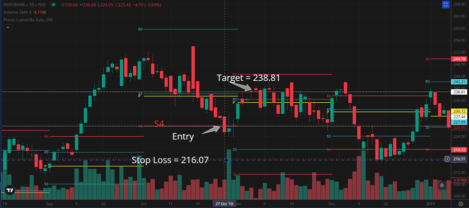
In our selected test sample, the trade occurred on October 27, 2010. The Buy Price is 227.446. The Stop Loss is correctly calculated as 216.0737, and the Target is 238.81. By examining the charts of HDFC Bank, we observe that the target level of 238.81 was surpassed on November 4, 2010. Since the Stop Loss was not triggered before this date, the Fixed Gains column, which records the profit or loss booked by the trading bot, is set to 5% for this trade. The maximum gains in the first 5 calendar days occurred on November 1. The high price on November 1 was 236.6. Let's verify the maximum gains in five days using a calculator: ((236.6−227.446)/227.446)×100=4.0246915, which matches our trading data output given by the code.
I have verified various other rows in a similar manner. This type of verification helps you understand if the code you developed is functioning as desired.
Output File:

Analysis of Trading Statistics around the buy point
Let's take a first look at the trading statistics generated around the buy point:
Fixed Gains Column: The average gains are 0.83%, with a total of 239 trades executed. The cumulative fixed gains amount to 200%.
Days to Gain Column: On average, trades were closed within 13 days from the buy price.
Days to Stop Loss Column: On average, the stop loss was triggered within 15 days.
Max Gains Columns:
5-day gains averaged 4%.
10-day gains averaged 5.4%.
30-day gains averaged 8.78%.
120-day gains averaged 18%.
These statistics provide valuable initial insights into the performance of the trading bot based on the defined strategy.
Key Parameters for Trading Success
Trading success hinges on three pivotal parameters: position size per trade, hold time for gains, and the amount of gains. Visualize these parameters as forming a triangle, where the area of the triangle represents the outcome—either profit or loss. When multiple strategies are deployed concurrently, they generate numerous small triangles. Collectively, these small triangles shape the overall gains and equity curve for your quantitative trading endeavors.


Position Sizing:
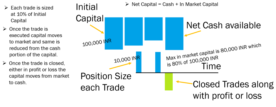
Let's implement this trading strategy by defining key parameters: position size, initial capital, and maximum capital usage at any given time. We'll start with an initial net capital of 100,000 INR in cash. The fixed position size will be 10,000 INR, which is 10% of the starting capital. Additionally, we'll cap the maximum capital usage at 80% of the net capital.
Here's a visual representation of the capital flow:
Net Available Cash: Represented by a large blue box, this is the cash you have on hand.
Executing a Trade: When a trade is executed with the defined position size of 10,000 INR, the net available cash decreases by that amount. This capital is then allocated to the market.
Capital in the Market: The cash portion of the capital decreases as it is invested in the market. The in-market capital is calculated daily based on the closing price for the day multiplied by the number of shares held.
Closing Trades: After trades are closed, whether they result in a profit or a loss, the capital returns to cash from the market. The net capital is the sum of the available cash and the in-market capital.
Key Points:
Initial Net Capital: 100,000 INR.
Fixed Position Size: 10,000 INR (10% of starting capital).
Maximum Capital Usage: 80% of net capital.
Net Available Cash: Decreases by the position size when a trade is executed.
In-Market Capital: Calculated daily based on the closing price and number of shares held.
Net Capital: Sum of available cash and in-market capital.
By carefully managing these parameters, you can effectively monitor and control your trading activities, ensuring that your capital is used efficiently and sustainably.
The eqCurveSample.py script executes trading activity based on the position sizing logic. For each trade, 10% of the initial capital is used, with a maximum capital usage capped at 80% of the total initial capital. The trading activity is driven by the buy and sell signals from the trading bot's CSV file. To determine the daily net value of the portfolio, we utilize the HDFC Bank daily OHLC (Open, High, Low, Close) values from a CSV file.
Upon running the Python script, a CSV file named HDFCBANK_daily_capital_analysis is generated. This file details the trading activity, including the date-wise capital used for trading, labelled as, In Market, cash available, and net capital values for each day.
For instance, the first trade occurred on July 24, 2000. The In Market Capital was approximately 9,964.72, Cash Available was 90,000, and the total net capital was around 99,964.72. The trade was closed the very next day at a profit, resulting in zero In Market capital, Cash Available of 100,499.47, and a corresponding Net Capital of 100,499.47.
By plotting the Net Capital chart, we can observe the capital growth over the years. Notably, by the end of the trading period, the capital had grown by 17% on an absolute basis, while the trading bot achieved approximately 170% gains based on position size.
I have uploaded the data to Datawrapper and created a chart visualization for a strategy with a -5% stop loss, 5% fixed gains, and a 48-day maximum hold period. By hovering over the chart, you can see how the In Market, Cash Available, and Net Capital values varied during the trading period.
Link to Datawrapper for above visualization: https://www.datawrapper.de/_/9A6Kf/
Next, let's optimize the parameters by tuning the Hold Time, Stop Loss percentage, and Fixed Gain percentage. After running the evaluateStrategy.py Python code, we obtain a CSV file that shows the strategy evaluation results. Let's open the output CSV file.
In this process, I varied the Stop Loss percent, Fixed Gains, and Hold Time to generate outputs such as the Sum of Fixed Gains, Average Fixed Gains, and Average R multiple. The R multiple represents the Risk to Reward ratio per trade. Averaging the R multiple values across all past backtested trades gives us the average R multiple for each set of input parameters.
Upon examining the results, we observe that the Average R multiple graph peaks at iteration number 22. By selecting the settings from iteration number 22—specifically, a Stop Loss of -3%, Fixed Gains of 18%, and a Hold Time of 60 days—we might achieve better gains, lower drawdowns, and more efficient capital usage.
Additionally, another promising iteration is number 96, with settings of a -12% Stop Loss, 18% Fixed Gains, and a 120-day Hold Time. This iteration boasts a relatively higher Average R multiple and similar high Fixed Gains.
These optimized parameters can help refine the strategy for improved performance.
Pyfolio for Backtesting
We will now run the Python code to generate the daily equity curve and then pass this output to Pyfolio to evaluate the backtest performance metrics. Pyfolio is a widely-used backtesting library available online. You need to install it in a separate conda environment. Once installed, you can run the code in Jupyter Notebook.
Here is the output file.
First, I passed HDFC Bank's close price returns data to Pyfolio to understand the stock's dynamics. The available data spans from May 9, 2000, to October 7, 2024, covering 289 trades. Here are the backtest performance metrics:
Annual return: Approximately 18.7%
Cumulative returns: 61 times the starting capital
Annual volatility: 29.9%
Sharpe ratio: Around 0.72
Max Drawdown: -55.4%
The severe max drawdown of -55.4% indicates extreme fluctuations in the portfolio's net value throughout the trading journey, which can be very challenging for typical investors to tolerate. Additionally, there is uncertainty about the stock's recovery from such significant falls. This scenario underscores the advantage of quantitative trading or setup-based trading in maintaining the linearity of the equity curve and reducing portfolio volatility. The underwater plots reveal several instances of drawdowns exceeding 30%.
Next, I passed the equity curve of net capital generated by trading using the settings of a -3% stop loss, 18% fixed gains, and a 60-day hold time:
Annual returns: 1.6%
Cumulative returns: 46.4%
Max drawdown: Limited to -7.1%
Focusing on the period from 2008 to 2012, when the buy-and-hold strategy faced a 55% drawdown, our strategy settings resulted in approximately 15% gains. The rolling Sharpe ratio reached as high as 4, and during the market crisis, the strategy's underwater level was less than 7%.
Lastly, I tested the settings of a -12% stop loss, 18% fixed gains, and a 120-day hold time:
Annual returns: 3.3%
Cumulative returns: 117.5%
Max drawdown: -17.2%
This setting achieved much better overall returns at the cost of higher drawdown. The cumulative returns graph shows a stable and upward-trending equity curve throughout the trading journey. During the 2008 to 2012 market crisis, the portfolio's underwater level was less than -8%, and the gains were around 23% during this period.
These results highlight the effectiveness of different trading strategies in managing risk and maximizing returns, especially during periods of market volatility.
To get the python code for above, subscribe here by sharing your email ID. You shall receive the link to code on your email.


Comments